I am jotting 5 excel quick hacks to perform Forensic Audit in Excel envoronment.
1) Identifying
Duplicate Transactions using Highlight Values:
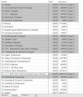
Consider the following
instance where we have a supplier name or code, supplier invoice number and the
amount. There is a chance that one might have a duplicate amount number or
duplicate invoice number for different suppliers – but what if a pair of
records have exactly the same data for all the three parameters? This is
a definite case of duplicate invoices existing:
In the above example we
have produced the column D by concatenating the data in the first three columns
and then applying the conditional formatting for duplicate values. (The
exact formula is =A2&B2&C2 in cell D2 and then dragged down, the
conditional formatting on cell D2:D13 can be applied by accessing Highlight
Values Menu from Home Tab.)
As you can see from this
screenshot, various duplicates are highlighted in the second and the third
column as well as the fourth column. We can ignore the duplicates in the
second and third column as invoice number and amount could be the same for
different suppliers – but the duplicate value in the fourth column means that
all the three parameters are the same. This points to a definite
duplicate entry that should be checked.
2) Analyzing
Round Numbered Transactions:
If a forensic accountant
is getting too many round numbers, it is time to check the accuracy of the
document or ask for further support. Too many round numbers may indicate
something fraudulent is occurring.
Excel has a built in
function called MOD () to analyze if a number is a round number or not.
The dynamics of the formula are simple – we add the following formula in the
example sheet to find if the number has to be checked for something potentially
fraudulent:
=IF(MOD(A2,100)=0,”Check”,”-“)
The formula will return a
non-zero number and the result can be presented as-is or nested into an IF()
statement to give the desired result:
3) Above
Average Payments to Vendors or Checking the Ratio between a Maximum and
Minimum:
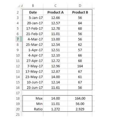
For a product, prices
usually fall within historical ranges. If anything goes beyond the
average, the entry can be question and should be verified. Consider data
in the following table that has price listed for two different products.
These products are bought over a period of six months and their prices vary between
a minimum of 11.01 and a maximum of 14, whereas the ratio of the max/min is
1.272. Compared to this, if we look at the second product, we find this
ratio to be 2.9 times or almost 3 times. This points to a discrepancy.
4) Gap
Detection:
This is a test that uses
a simple fact that any missing invoice (number) in the sales database can
indicate a potential problem. This test can be done for such a document
and help drive for further inquiry of the preparer.
In excel we can do this
test by first sorting the invoice number and then taking the difference of
consecutive invoices. The following screenshot how the excel sheet is
setup for this case:
In the above example, we
have setup a formula that calculate the difference between the two consecutive
invoice numbers, if it is one, then its okay and we move forward. If not,
it means that an invoice number was skipped – we can then write a conditional
formula with IF() that can give us a custom message like this:
=IF(A3-A2<>1,A3-A2-1&” – Invoice(s)
Missing”,”-“)
The above formula checks
if the difference is one, if not, we have a custom message that “n-invoices are
missing”. Otherwise, we will have a blank cell.
5) Checking
Ratio of the Highest to the Second Highest Number:
This is again a procedure
that relies on the use of finding maximum, but not just maximum but also the
second largest number in the data.
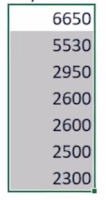
Consider the following
data for a part purchased from a supplier:
We can use build in
function MAX() and LARGE() to find the maximum and the second largest value in
the data. As we take the ratio of the data, we find it to be 10 times the
maximum number. This means that maximum for the data is much larger than the
usual average value.
Conclusion:
We cannot eliminate
mistakes or “fudging” in the financial data however we can positively try to
minimize it. We have seen five techniques that can be applied using a
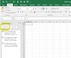
standard tool like MS Excel for tracing such issues. Please download the
attached file to see it working practically.


 It would temporary replace all values with formulas.